Machine Learning from Scratch: Principal Component Analysis

Introduction

In this post, I’ll be implementing Principal Component Analysis (PCA) from scratch in Python. This is the eighth post in the “Machine Learning from Scratch” series.

PCA is an unsupervised learning technique used for dimensionality reduction. It transforms high-dimensional data into a lower-dimensional space while preserving as much variance as possible.

Principal Component Analysis

PCA identifies the directions (principal components) along which the variance in the data is maximized. These components are orthogonal to each other and ordered by the amount of variance they explain.

The algorithm works as follows:

1. Standardize the data by subtracting the mean
2. Compute the covariance matrix
3. Calculate eigenvectors and eigenvalues of the covariance matrix
4. Sort eigenvectors by eigenvalues in descending order
5. Select the top k eigenvectors as principal components
6. Transform the data by projecting it onto these components

PCA is widely used for visualization, noise reduction, and as a preprocessing step before applying other machine learning algorithms.

Implementation

I’m using numpy for numerical computations. For testing, I’ll use the Iris dataset from scikit-learn and reduce it from 4 dimensions to 2 for visualization.

The PCA class has the following methods:

• __init__: Constructor to set the number of components.
• fit: Method to compute principal components from the training data.
• transform: Method to project data onto the principal components.

import numpy as np
from sklearn import datasets
import matplotlib.pyplot as plt

class PCA:
    def __init__(self, n_components):
        self.n_components = n_components
        self.components = None
        self.mean = None

    def fit(self, X):
        self.mean = np.mean(X, axis=0)
        X = X - self.mean

        cov = np.cov(X.T)

        eigenvectors, eigenvalues = np.linalg.eig(cov)

        eigenvectors = eigenvectors.T

        idxs = np.argsort(eigenvalues)[::-1]
        eigenvalues = eigenvalues[idxs]
        eigenvectors = eigenvectors[idxs]

        self.components = eigenvectors[:self.n_components]

    def transform(self, X):
        X = X - self.mean
        return np.dot(X, self.components.T)

Now let’s test PCA on the Iris dataset by reducing it from 4 dimensions to 2.

if __name__ == '__main__':
    data = datasets.load_iris()
    X = data.data
    y = data.target

    pca = PCA(n_components=2)
    pca.fit(X)
    X_projected = pca.transform(X)

    print(f"Original shape: {X.shape}")
    print(f"Transformed shape: {X_projected.shape}")

    fig = plt.figure(figsize=(8, 6))
    plt.scatter(
        X_projected[:, 0], X_projected[:, 1], 
        c=y, cmap='viridis', s=40
    )
    plt.xlabel('First Principal Component')
    plt.ylabel('Second Principal Component')
    plt.show()

Let’s visualize the dimensionality reduction:

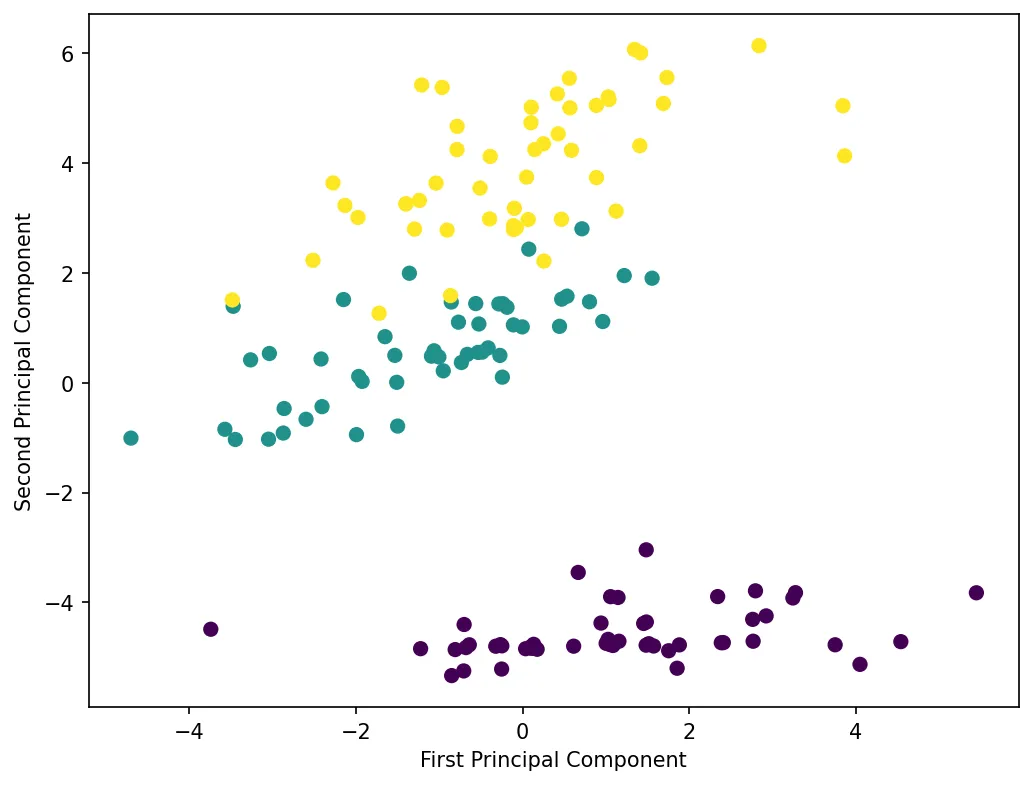
The plot shows the Iris dataset projected onto its first two principal components. Despite reducing from 4 dimensions to 2, the three species remain well-separated, demonstrating that PCA preserved the important structure in the data.

That’s all for this post. Thanks for reading!